Connect 4 GamePlay AI & Computer Vision System

Hello, my name is Martin Tin. I am a Grade 10 student at TMS Schools. As an IB MYP (Middle Years Programme) student, I had to do the Personal Project, a passion project. For this project, I created a connect 4 gameplay AI (MCTS) and computer vision framework for playing connect 4 with AI in-real-life.

• The computer vision component, based off a framework devised by Matt Jennings, allows the computer to read the state of a real-world board.
• The gameplay AI is a hard-coded version of Monte Carlo Tree Search. (MCTS) which provides the best piece placement denoted by the blue-edged piece on the display.

Implementing Connect 4:

Before implementing MCTS, I had to create a Connect 4 framework to apply the algorithm to.This involved the creation of a game board class which represents the Connect 4 board as a 2d array where board[y][x] is the position on the y-th row and x-th column and board[0][0] is the top-left corner position. As array indexing starts at 0, the row 0 and column 0 are the 1st row and 1st column.

In a typical connect 4 board, different player pieces are represented by different colors. (e.g. red and yellow) My implementation uses numbers (1 and 2) to represent this. 0 represents an empty position.

This game class also contains several methods:

getBoard()

• getBoard() returns the game board state

printBoard()

• printBoard() prints the board in console

setBoard(new_board)

• setBoard() changes the game board to the new_board argument

move(symbol,col)

• move() accepts two arguments: symbol and col. (column) move() is responsible for making a move and returning the resulting game state.

checkStraight(board,x,y)

• checkStraight() accepts a board argument and checks if there is a column of 4 repeating symbols (known as connect 4) extending from board[y][x]. If a connect 4 is detected, checkStraight returns True. Otherwise it returns False.

checkDiagonal(board,x,y)

• checkDiagonal() accepts a board argument and checks if there is a diagonal connect 4 with the bottom-left corner being board[y][x]. If a connect 4 is detected, checkDiagonal() returns True. Otherwise it returns False.

isTerminal()

isTerminal() rotates the board 3 times and uses checkDiagonal() and checkStraight() on every valid x,y coordinate to comprehensively check for wins or loses. If no positions are empty, it determines that a tie has been reached. isTerminal() returns the game status (True for a game end, False otherwise) followed by the symbol of the winner. If the game has been won by someone, the winning symbol is returned. If the game is tied, the string “TIE” is returned. Otherwise, 0 is returned.

getLegalActions()

getLegalActions() takes the current game state and returns all possible actions from the game state.

Tree Data-Structure:

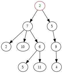
In computer science, a tree is an acyclic undirected graph data structure. Simply put, a data structure is a method of organizing and storing data. Trees are made out of nodes. A node is a structure which contains information used to represent a particular concept, thing or idea. Nodes can be connected to other nodes. In the Connect 4 implementation of MCTS, nodes represent a particular game board state and a two-node connection would represent that one node’s state can be reached from the other by one move. Nodes can be classified in reference to other nodes. The four main types of classifications are parent nodes and child nodes:

Parent/child nodes:

A parent node is connected to its child nodes. A parent node is considered superior to its child nodes. This superiority can represent different ideas. In our Connect 4 MCTS tree, a parent node represents a particular game state and its children are all of the game states reachable in one move from the parent.

Root node:

In a tree, there is only one root node. The root node is the only node that does not have a parent node. All nodes of a tree can be traversed using the root node’s children.

Terminal node:

A terminal node is a node that cannot have any children. In our Connect 4 situation, this means that the game state of a terminal node is at a win/loose or tie position. Thus, no further moves can be applied to reach a child state.

Introduction to Monte Carlo Tree Search (MCTS):

Monte Carlo Tree Search or MCTS is a computational algorithm most known for its uses in board game AI. Notably, in 2016, a neural network-MCTS hybrid was used to master the game of Go. It is a search algorithm which builds an asynchronous game tree based off random sampling. In fact, the “Monte Carlo” part of Monte Carlo Tree Search comes from the term Monte Carlo methods which are a grouping of algorithms which use random sampling to solve problems.

Essentially, the gist of MCTS is to run a bunch of simulations and determine the best decision given the probabilities of success it receives from those simulations. Using the context of Connect 4, MCTS would take a game state and output the best move possible based off the probabilities of thousands of gameplay simulations.

Although MCTS might seem intimidating at first, it can be easily understood by breaking the process into steps. For MCTS, an operation known as a play-out is repeated until the decision tree has successfully gathered enough information. A play-out, also known as a roll-out, expands the game tree with simulations.

The play-out process is made of multiple steps: selection, expansion, simulation and backpropagation.

Selection:

Before I explain selection, I must warn you, the reader, that I will mention the Upper Confidence Bound 1 (UCB1) algorithm and UCB1 value. Do not fret! This will be explained later. For now, just keep in mind that the node with the highest UCB1 value is considered the “best move.”

In any case, selection begins at node N. If all of node N’s children have been simulated at least once, select the child node of N with the highest UCB1 value. Continue selection like this until a node is encounter with an un-simulated child node. Denote this child node as K. If there are multiple un-simulated child nodes, K can be chosen arbitrarily from them.

select() evaluates the UCB1 values of all of the current node’s children and returns the child with the highest UCB1 value.

select() is applied to a while loop which constantly iterates until a terminal node is reached or the current node has an un-simulated child. For now, you can ignore the contents of the if block. Just know that if a terminal node is reached, the selection/expansion steps are skipped and backpropagation occurs. These terms will be explained.

Expansion:

Expansion occurs after node K has been chosen. A child node C is arbitrarily created from K.

Simulation:

From Node C select a random, valid move. Continue selecting until the game has been resolved. (win, draw, loss)

Backpropogation:

Record the results of simulation. Backtrack to node R and for each node encountered, adjust their win, draw, loss counter accordingly.

UCB1:

UCB1 or Upper Confidence Bound is MCTS’ solution to the exploration vs exploitation challenge. This is a consequence of MCTS being a learning algorithm for multi-armed bandit problems. Multi-armed bandit problems are a classification of different scenarios which share a common underlying problem.

Consider a scenario where there is a row of 20 casino slot machines. You have 100 casino tokens to spend on any of these 20 slot machines. When a player wins, all machines return $100. However, the probability distribution of winning differs between all machines. Now, you have to develop a learning strategy which gains the most money using your 100 tokens.

The inherent challenge with this is that the relative probability distribution of a machine can only determined by simulation. Consequently, better slot machines can only be found by using your tokens on new slot machines. This process is known as exploration. By engaging in exploration, it is true that better slot machines can be found. However, by exploring, we cannot exploit our previous findings. For example, let’s say you have used tokens on the first 5 machines and determined, with relative confidence, how often each slot machine returns a reward. By doing so, we are able to establish the best possible slot machine out of the five. When we explore other slot machines with undetermined reward yields, we may be wasting our tokens with worse machines. By not exploiting our current knowledge and spending tokens on the best machine out of the first few, we would earn less. Alternatively, we could also discover a better slot machine however, by not spending our tokens on a machine we know is relatively good, we could still earn less.

In MCTS, each slot machine represents a game state node of the game decision tree. The tokens represent the maximum amount of play-outs. Thus, the exploitation vs exploration problem in MCTS is distilled into the challenge of saving time through the optimal use of simulations to develop the game tree.

In training, a node with a higher UCB1 value should be visited over a node with a lower UCB1 value. The UCB1 value of a machine changes every time it is used. Here is the formula:

wi = number of wins of node

ni = number of simulations of node

Ni = number of simulations of the node’s parent

c = exploration parameter

The first term of UCB1 is known as the “average reward.” It represent the probability of the node winning. The higher the probability, the higher the UCB1 value.The second term is known as the confidence interval for exploration. It is higher for node’s with fewer simulations.

Mathematically, the exploration parameter is sqrt(2) however, it is often chosen by the repetitive testing of MCTS.

An important distinction is that UCB1 values are not used for final decision making. Rather, during training, the UCB1 values guide the MCTS algorithm into simulating the best nodes more frequently. Thus, the number of simulations or visits of a node correlates with the established likelihood of winning from that node.

Full Code:

Here it is! This is my full Python implementation of MCTS! It creates a new game tree on its turn and discards the game tree after each move.

Importantly, my implementation decides it has run enough play through based off how many nodes have been explored. However, other implementation have also used a timed approach where the number of play-throughs is limited by time.

=

connect4_ai/mcts.py at main · tin-martin/connect4_ai

MCTS: Advantages vs Disadvantages:

Unlike mini-max, MCTS is very interesting in that it requires no heuristics. Heuristics are success criteria which inform the algorithm on Essentially, heuristics are. Heuristics do lessen the training cost of an algorithm however, heuristic-based algorithms tend to fail in situations where success criteria becomes hard to define. An example is Go where there are a multitudinous amount of strategies of move-placements. This is where MCTS finds its niche; it was specifically designed for these situations where an algorithm is forced to “define” what is successful.

When considering the “pros” vs “cons” of MCTS, it becomes evident that the choice of MCTS was not a good decision for connect4 where there are proven strategies simple enough for a human to follow. My experience with training MCTS has corroborated this as it admittedly does take quite a while to develop some notion of a good move.

Before I engaged in this project, I assumed that vanilla MCTS would be able to overcome its inherent training difficulties and demonstrate complex behaviours. I attempted to set out and either prove or disprove this hypothesis. However, my results are inconclusive. Although my MCTS algorithm performed poorly relative to my expectations, I cannot definitively state that this is the case for other implementations.

Thinking back, I believe there would’ve been several better approaches to applying MCTS:

1. Retain the same game tree and use a pathfinding algorithm (like Breadth First Search (BFS) or Depth First Search( DFS) ) to locate the game state returned by the opponent.
2. A single pre-trained game tree compiled over billions of simulations could be used to identify every possible move. This is similar to the mini-max framework by Pascal Pons.